Training a Gaussian Process from an AIMD Run¶

Steven Torrisi (torrisi@g.harvard.edu), December 2019

In this tutorial, we’ll demonstrate how a previously existing Ab-Initio Molecular Dynamics (AIMD) trajectory can be used to train a Gaussian Process model.

We can use a very short trajectory for a very simple molecule which is already included in the test files in order to demonstrate how to set up and run the code. The trajectory this tutorial focuses on involves a few frames of the molecule Methanol vibrating about its equilibrium configuration ran in VASP.

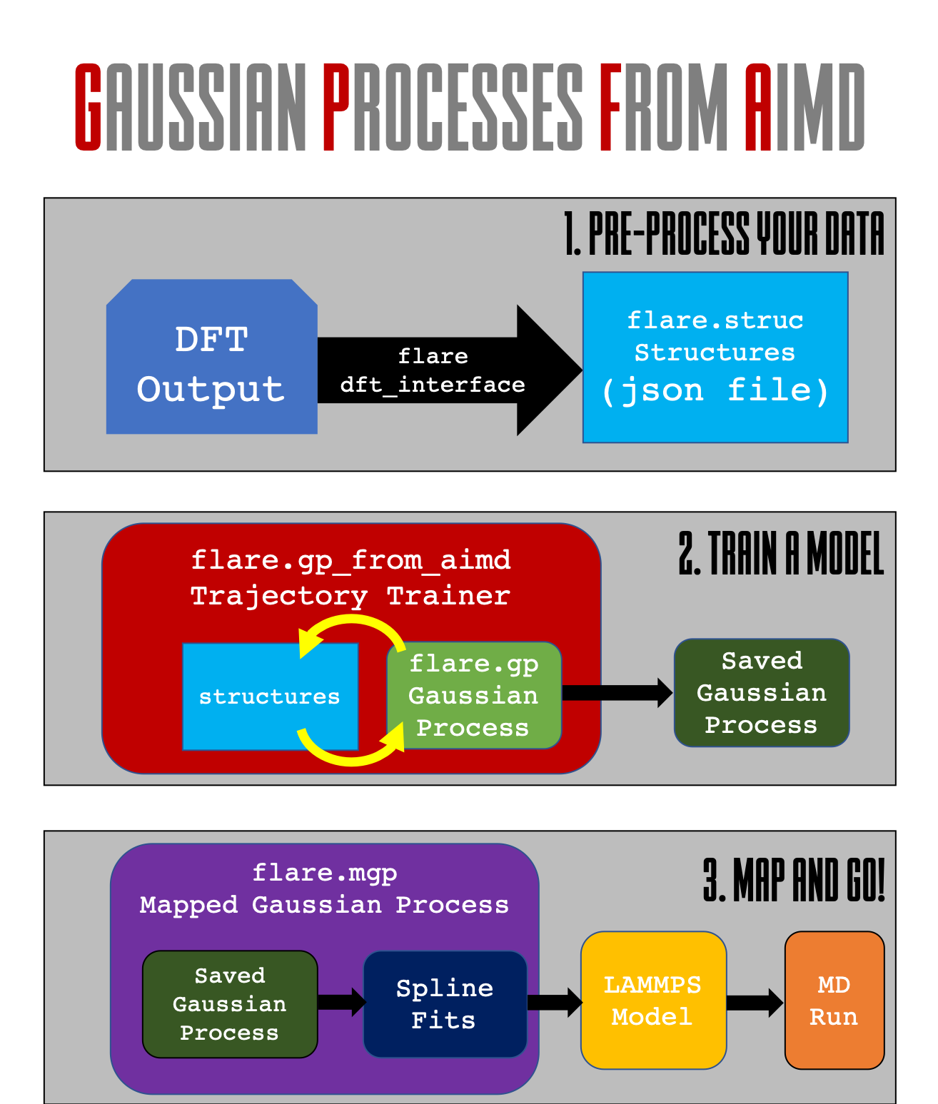
Roadmap Figure¶

In this tutorial, we will walk through the first two steps contained in the below figure. the GP from AIMD module is designed to give you the tools necessary to extract FLARE structures from a previously existing molecular dynamics run.

Step 1: Setting up a Gaussian Process Object¶

Our goal is to train a GP, which first must be instantiated with a set of parameters.

For the sake of this example, which is a molecule, we will use a two-plus-three body kernel. We must provide the kernel name to the GP, “two-plus-three-mc” or “2+3mc’. Our initial guesses for the hyperparameters are not important. The hyperparameter labels are included below for later output. The system contains a small number of atoms, so we choose a relatively smaller 2-body cutoff (7 A) and a relatively large 3-body cutoff (7 A), both of which will completely contain the molecule.

At the header of a file, include the following imports:

from flare.gp import GaussianProcess

We will then set up the GaussianProcess object.

The GaussianProcess object class contains the methods which, from an

AtomicEnvironment object, predict the corresponding forces and

uncertainties by comparing the atomic environment to each environment in the

training set. The kernel we will use has 5 hyperparameters and requires two cutoffs.
The first four hyperparameters correspond to the signal variance and length

scale which parameterize the two- and three-body comparison

functions. These hyperparameters will be optimized later once data has

been fed into the GaussianProcess via likelihood maximization. The

fifth and final hyperparameter is the noise variance. We provide simple

initial guesses for each hyperparameter.
The two cutoff values correspond to the functions which set up

the two- and three-body Atomic Environments. Since Methanol is a small

molecule, 7 Angstrom each will be sufficent.
The kernel name must contain the terms you want to use.
Here, we will use the two_plus_three_body_mc kernel, which

uses two-body and three-body comparisons. mc means multi-component,

indicating that it can handle multiple atomic species being present.

gp = GaussianProcess(kernels=['twobody', 'threebody'],
hyps=[0.01, 0.01, 0.01, 0.01, 0.01],
cutoffs = {'twobody':7, 'threebody':3},
hyp_labels=['Two-Body Signal Variance','Two-Body Length Scale','Three-Body Signal Variance',
'Three-Body Length Scale', 'Noise Variance']
                )

Step 2 (Optional): Extracting the Frames from a previous AIMD Run¶

FLARE offers a variety of modules for converting DFT outputs into FLARE structures, which are then usable for model training and prediction tasks. For this example, we highlight the vasp_util module, which has a function called md_trajectory_from_vasprun, which can convert a vasprun.xml file into a list of FLARE Structure objects, using internal methods which call pymatgen’s IO functionality.

You can run it simply by calling the function on a file like so:

from flare.dft_interface.vasp_util import md_trajectory_from_vasprun
trajectory = md_trajectory_from_vasprun('path-to-vasprun')

Step 3: Training your Gaussian Process¶

If you don’t have a previously existing Vasprun, you can also use the one available in the test_files directory, which is methanol_frames.json. You can open it via the command

from json import loads
from flare.struc import Structure
with open('path-to-methanol-frames','r') as f:
        loaded_dicts = [loads(line) for line in f.readlines()]
trajectory = [Structure.from_dict(d) for d in loaded_dicts]

Our trajectory is a list of FLARE structures, each of which is decorated with forces.

Once you have your trajectory and your GaussianProcess which has not seen any data yet, you are ready to begin your training!

We will next import the dedicated TrajectoryTrainer class, which has a variety of useful tools to help train your GaussianProcess.

The Trajectory Trainer has a large number of arguments which can be passed to it in order to give you a fine degree of control over how your model is trained. Here, we will pass in the following:

frames: A list of FLARE ``structure``s decorated with forces. Ultimately,

these structures will be iterated over and will be used to train the model.
gp: Our GaussianProcess object. The process of training will involve

populating the training set with representative atomic environments and

optimizing the hyperparameters via likelihood maximization to best explain

the data.

Input arguments for training include:

rel_std_tolerance: The noise variance heuristically describes the amount

of variance in force predictions which cannot be explained by the model.

Once optimized, it provides a natural length scale for the degree of

uncertainty expected in force predictions. A high uncertainty on a force

prediction indicates that the AtomicEnvironment used is

significantly different from all of the ``AtomicEnvironment``s in the training

set. The criteria for adding atoms to the training set therefore be

defined with respect to the noise variance: if we denote the noise variance

of the model as sig_n, stored at gp.hyps[-1] by convention, then the

the cutoff value used will be

rel_std_tolerance * sig_n. Here, we will set it to 3.
abs_std_tolerance: The above value describes a cutoff uncertainty which

is defined with respect to the data set. In some cases it may be desirable

to have a stringent cutoff which is invariant to the hyperparameters, in

which case, if the uncertainty on any force prediction rises above

abs_std_tolerance the associated atom will be added to the training set.

Here, we will set it to 0. If both are defined, the lower of the two will be

used.

Pre-Training arguments¶

When the training set contains a low diversity of atomic configurations relative to what you expect to see at test time, the hyperparameters may not be representative; furthermore, the training process when using rel_std_tolerance will depend on the hyperparameters, so it is desirable to have a training set with a baseline number of ``AtomicEnvironment``s before commencing training.

Therefore, we provide a variety of arguments to ‘seed’ the training set before commencing the full iteration over all of the frames passed into the function. By default, all of the atoms in the seed frames will be added to the training set. This is acceptable for small molecules, but you may want to use a more selective subset of atoms for large unit cells.

For now, we will only show one argument to seed frames for simplicity.

pre_train_on_skips: Slice the input frames via

frames[::pre_train_on_skips]; use those frames as seed frames. For

instance, if we used pre_train_on_skips=5 then we would use every fifth

frame in the trajectory as a seed frame.

from flare.gp_from_aimd import TrajectoryTrainer
TT = TrajectoryTrainer(frames=trajectory,
                    gp = gp,
                    rel_std_tolerance = 3,
                    abs_std_tolerance=0,
                    pre_train_on_skips=5)

After this, all you need to do is call the run method!

TT.run()
print("Done!")

The results, by default, will be stored in gp_from_aimd.out, as well as a variety of other output files. The resultant model will be stored in a .json file format which can be later loaded using the GaussianProcess.from_dict() method.

Each frame will output the mae per species, which can be helpful for diagnosing if an individual species will be problematic (for example, you may find that an organic adsorbate on a metallic surface has a higher error, requiring more representative data for the dataset).