Formulation of Mapped Gaussian Process¶

We take 2-body kernel as an example, for the simplicity of explanation. The local environment to be predicted is denoted as $\rho_i$ , which consists of a center atom $i$ whose force is to be predicted, and all its neighbors within a certain cutoff.

Energy¶

The atomic energy of $\rho_i$ from Gaussian Process regression is

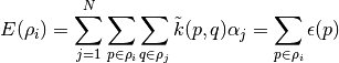
$\begin{aligned} E(\rho_i) = \sum_{j=1}^N \sum_{p \in \rho_i} \sum_{q\in \rho_j}\tilde{k}(p, q)\alpha_j = \sum_{p \in \rho_i}\epsilon(p) \end{aligned}$

where in 2-body, $p$ is a bond in $\rho_i$ , and $q$ is a bond in training data 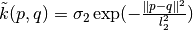$\rho_j$ , $\tilde{k}(p,q)=\sigma_2\exp(-{\|p-q\|^2\over l_2^2})$ is the kernel function. $\boldsymbol{\alpha}=\mathbf{\Sigma}^{-1}\mathbf{y}$ is the inverse kernel matrix multiplied by the label vector (forces of the training set).

In the equation above, we can see that the atomic energy can be decomposed into the summation of the bond energies $\epsilon(p)$ , which is a low dimension function, for n-body kernel, its dimensionality of domain is ${n(n-1)\over 2}$ . Therefore, we use a cubic spline to interpolate this function, with a GP model with fixed training data and hyperparameters. The forces can be derived from the derivative of the above function.

While in GP, the triple summations are needed in prediction, after mapping to the cubic spline, the two summations w.r.t. the training data set $\sum_{j=1}^N \sum_{q\in \rho_j}$ are removed. The computational cost in prediction of GP scales linearly w.r.t. the training set size $N$ due to the two summations, and MGP is independent of $N$ .

Uncertainty¶

The atomic uncertainty of $\rho$ from Gaussian Process regression is

$V(\rho) = \sum_{p\in \rho, q \in \rho} V(p, q)$

$V(p, q) = \tilde{k}(p, q) - \sum_{i,j} \sum_{u\in \rho_i, v\in \rho_j} \tilde{k}(p, u) (\Sigma^{-1})_{ij} \tilde{k}(v, q)$

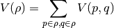
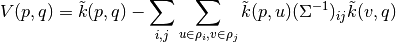
Since $V(p,q)$ has twice the dimensionality of domain compared with $\epsilon(p)$ , it will be expensive both in computational cost and memory if we want to interpolate $V(p,q)$ directly with spline function, because a large number of grid points are needed for interpolation. To solve this problem, we observe that the 2nd term expressed in vector form is:

$\tilde{\mathbf{k}}^\top(p)\Sigma^{-1} \tilde{\mathbf{k}}(q) = \left(\tilde{\mathbf{k}}^\top(p)L^{-\top}\right) \left(L^{-1} \tilde{\mathbf{k}}(q)\right) := \boldsymbol{\psi}(p)^\top \boldsymbol{\psi}(q)$

$L$ : Cholesky decomposition of matrix $\Sigma$ , and define 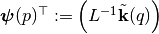$\boldsymbol{\psi}(p)^\top := \left(L^{-1} \tilde{\mathbf{k}}(q)\right)$ . The GP variance

$V(p,q) = \tilde{k}(p,q) - \boldsymbol{\psi}(p)^\top \boldsymbol{\psi}(q)$

Then we use splines to map the vector function 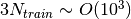$\boldsymbol{\psi}(p)$ . Notice $\boldsymbol{\psi}(p)$ has $3N_{train}\sim O(10^3)$ components. Have to build $3N_{train}$ maps $\to$ too many!

Dimension reduction¶

Can we find $m$ -component vector function $\boldsymbol{\phi}(p)$ ( $m$ is small), such that

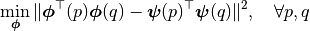
$\min_{\boldsymbol{\phi}} \|\boldsymbol{\phi}^\top(p)\boldsymbol{\phi}(q) - \boldsymbol{\psi}(p)^\top \boldsymbol{\psi}(q)\|^2, \quad \forall p, q$

Then we can estimate the variance as

$V(p,q) = \tilde{k}(p,q) - \boldsymbol{\phi}(p)^\top \boldsymbol{\phi}(q)$

and only build $m$ maps instead of $3N_{train}$

Principle component analysis (PCA) is what we want
We can pick up any $m$ by picking up the rank in PCA, the higher rank, the better estimation

References¶

[1] Xie, Yu, et al. “Fast Bayesian Force Fields from Active Learning: Study of Inter-Dimensional Transformation of Stanene.” arXiv preprint arXiv:2008.11796 (2020).

[2] Glielmo, Aldo, Claudio Zeni, and Alessandro De Vita. “Efficient nonparametric n-body force fields from machine learning.” Physical Review B 97.18 (2018): 184307.

[3] Glielmo, Aldo, et al. “Building nonparametric n-body force fields using gaussian process regression.” Machine Learning Meets Quantum Physics. Springer, Cham, 2020. 67-98.

[4] Vandermause, Jonathan, et al. “On-the-fly active learning of interpretable Bayesian force fields for atomistic rare events.” npj Computational Materials 6.1 (2020): 1-11.